I thus decided to get a little coding exercise by implementing a version of the FM Index data structure and using it to search the Adobe data. I finally got round to finishing my implementation a month or so ago. The source (written in C++ and wrapped for python in Cython) is available here. Using this code, I can perform substring searches that previously took over two minutes in a few microseconds (a speed-up factor of nearly 108 in many cases).
I have written this post in large part for my future myself and the level of detail varies from place to place according to the peculiarities of my ignorance but I still hope it may be of interest to others. Any feedback will be gratefully received.
A typical record from the leaked data looks something like this:
103238703-|-usually_blank_user_id-|-adobe_breach_example@gmail.com-|-Mai82+/AmfZ=-|-my cat's birthday|--
The three fields of interest in the above are:

(The reason for using a string ending in '$' will be explained below.)
The humble suffix array is extremely useful but it does have its disadvantages. These include:

We shall henceforth refer to this as the hypothetical matrix. The reason for including the extra '$' character can now be explained: since it is lexicographically smaller than all other characters in the string, the lexicographic order of the suffixes is the same as that of the cyclic permutations. We shall refer to strings terminated with a unique smallest letter as minimally-terminated.
A substring can be defined as a prefix of a cyclic permutation and thus corresponds to a (possibly-empty) set of consecutive rows of the hypothetical matrix. Suppose that for a given string we have the hypothetical matrix to hand and wish to look for a substring. There is a beautifully-simple inductive algorithm for finding the corresponding rows, due to Ferragina and Manzini, known as backward search.
Note first that it is trivial to find a length-1 substring. Since the hypothetical matrix is sorted lexicographically by rows, we just need to find the set of consecutive rows that start with the letter that is our length-1 substring. We can accomplish this in logarithmic time using binary search, but if we suppose that we have precomputed the cumulative letter frequencies in our alphabet, we can do it in constant time. More precisely, define an integer-valued function, \(C\) say, on our alphabet as follows: $$ C[x] = \mbox{number of letters of our string strictly less than $x$} $$ For example, \(C\) would take the following values for our string:

Even though it is trivial, we state the result we need formally for emphasis:
Proposition 1 [base case] Suppose we have an ordered alphabet, a distinguished letter \(x\) and a minimally-terminated length-n string over the alphabet. Using 0-based indexing, the set \(S_x\) of row indexes of the hypothetical matrix corresponding to the prefix x is the half-open interval: $$ S_x = [C[x], C[x']) $$ where \(x'\) is the next-largest character in the alphabet after \(x\) unless \(x\) is the maximal character in which case we read \(C[x']\) as \(n\).
The induction step is:
Proposition 2 [induction step] Suppose we have an ordered alphabet, a distinguished letter \(x\), a minimally-terminated string over the alphabet and a substring P that does not reach the terminating character. Suppose, using 0-based indexing, that the set SP of row indexes of the hypothetical matrix corresponding to prefix P is the half-open interval: $$ S_P = [lb, ub) $$ then the set \(S_{xP}\) of rows of the hypothetical matrix corresponding to prefix \(xP\) is the half-open interval: $$ S_{xP} = [lb', ub') $$ where: $$ lb' = C[x] + rank(x, lb-1)\\ ub' = C[x] + rank(x, ub-1) $$ and \(rank(x, i)\) is the number of occurrences of the letter x in the right-most column of the hypothetical matrix with row index at most \(i\). Furthermore, the above remains correct even if \( lb' \ge ub'\) since this happens iff \(xP\) is not a substring.
This innocent-looking proposition (whose proof we shall outline below) is extremely useful. Perhaps most importantly, it means that although we have been assuming we have the entire hypothetical matrix to hand, we can identify the rows corresponding to a substring using only the data of the left-most column (encoded as \(C\)) and the right-most column. In fact the right-most column is so important that it has its own name.
Definition The right-most column of the hypothetical matrix associated to a minimally-terminated string is known as the Burrows-Wheeler Transform of that string.
For example the Burrows-Wheeler Transform of cohomology$ is y$oooolcmhg. The transform was originally invented as an aid for text compression (it is used by bzip2 for example). As we shall see below, one can recover a string from its Burrows-Wheeler Transform and it tends to rearrange letters in a way that is more friendly to many compression techniques. It can thus provide a useful pre-compression transformation. Unlike the vast majority of text compression ideas, the Burrows-Wheeler transform is global in nature, making it a powerful complementary technique.
It is time to outline a proof of proposition 2.
Consider what we know about the hypothetical matrix under the hypotheses of proposition 2. Assuming for simplicity that xP is indeed a substring, the hypothetical matrix will look like this:

This follows from the fact that the rows of the hypothetical matrix are simply the set of all cyclic permutations of the given string.
Recalling the definition of the rank function from proposition 2, we complete the argument by noting that because the hypothetical matrix is sorted lexicographically by rows: $$ rank(x, i-1) = \mbox{the number of rows of the form Q...x with } Q < P \mbox{ lexicographically} $$ where \(i\) is the index of the first row beginning with \(P\). We thus arrive at the formula for \(lb'\) stated in proposition 2. A similar argument deals with \(ub'\) and a little case analysis shows that the results hold in the generality stated.
Just before we describe the FM Index data structure that is built around the backward search algorithm, it is worth highlighting this blog post of Alex Bowe. Amongst other things, Bowe has some superb pictures illustrating backward search.
If we have the suffix array to hand, the values of the suffix array at the row indexes provided by backward search will be the indexes of where the substring occurs in the text. Thus if we store both the suffix array and the Burrows-Wheeler Transform of the text, we can answer the substring problem very efficiently (we shall see below that it is easy to store the Burrows-Wheeler Transform in such a way that the required rank queries can be performed in constant time with good constant factors). However storing the suffix array does not escape the disadvantage that it usually takes up several multiples as much space as the text. For this reason, Ferragina and Manzini suggested storing only one in k values of the suffix array for some chosen value of k, such that the values are evenly-spaced in the text. That this sampled suffix array is still sufficient to locate substrings of the text (albeit with a mild time penalty) is a consequence of the following:
Proposition 3 If the \(i\)th letter of the Burrows-Wheeler Transform of a minimally-terminated string \(T\) is \(m\)th letter of \(T (m > 0)\) and we set: $$ x = select(i)\\ j = C[x] + rank(x, i) $$ where \(select(i)\) is the function that returns the \(i\)th letter of the Burrows-Wheeler Transform, then the \(j\)th letter of the Burrows-Wheeler Transform is the \((m-1)\)th letter of \(T\).
The proof follows easily by reasoning along lines used to establish proposition 2 above.
This extremely useful property of the Burrows-Wheeler Transform means that we can iterate backwards in the text using only its Burrows-Wheeler Transform and that provided we can answer both rank and select queries in constant time, each step takes only constant time. (This also shows that we can recover a string from its Burrows-Wheeler Transform, though there are easier ways of seeing this.) In particular we see that the sampled suffix array approach suggested by Ferragina and Manzini enables us to locate substrings with only an additive \(O(k)\) time penalty vs. storing the entire suffix array (iterate backwards till at one of the sampled values of the suffix array and then report the value found plus the number of steps taken).
Finally we note that there is no efficient algorithm for iterating forward in the text using its Burrows-Wheeler Transform. This asymmetry is due to the fact that the lexicographic sorting used to construct the hypothetical matrix is left-to-right. If we were to sort right-to-left, we would have the opposite asymmetry. A moment's thought reveals this is really just the same the Burrows-Wheeler Transform of the reversed text. We will make use of this below.
As we have seen, iterating backward is not a problem, but iterating forward is. There are multiple solutions to this problem but I felt the most natural approach was to store the Burrows-Wheeler Transform of both the text and its reverse. This doubles the memory requirement but gives us the ability to iterate in either direction in the text.
Unfortunately what the above approach gives us is unidirectional iteration in either direction but not bidirectional iteration, which is really what we need. The problem is that locations in the Burrows-Wheeler Transform of the text and its reverse do not naturally correspond. They each give row indexes, but into different hypothetical matrices: the rows are differently permuted. Storing the permutation that lines up indexes into the Burrows-Wheeler Transform of the text and its reverse would be too memory hungry so we need a way to compute this on the fly.
To solve this problem, I took advantage of the fact that for the ordering of the row indexes obtained by performing backward search on the Burrows-Wheeler Transform of the text, the contexts after each occurrence of the sought-for pattern are sorted in increasing lexicographic order. The corresponding ordering of the row indexes obtained by performing backward search on Burrows-Wheeler Transform of the reversed text can thus be obtained by sorting these according to this context. A most-significant-digit radix-sort fit the problem well and usually takes sub-linear time to complete.
Notwithstanding the above, I should point out that when there are large numbers of occurrences of the sought-for pattern, the sorting does become a bottleneck even though it is asymptotically optimal.
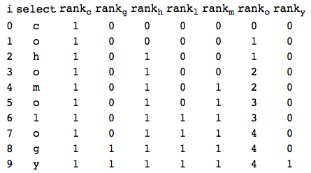
select takes an index into position in the string and returns the letter at that location. rank takes an index into a position in the string as well as a letter from the alphabet and returns the number of occurrences of that letter in the string, up to and including that location.
The following table provides some examples:
The catchy name is a bit misleading (there is a very weak analogy with some techniques used to perform the Wavelet Transform) but the idea is extremely appealing, very useful and astonishingly recent. Wavelet Trees were introduced in the SODA 2003 paper of Grossi, Gupta, Vitter, "High-Order Entropy-Compressed Text Indexes".
The easiest way to explain the idea, is to start with a picture:

The blue text is present solely for purposes of explanation; the tree stores only the data in red. This data in red consist of a bit vector and an ordered alphabet. The tree is defined recursively as follows.
Given a string over an ordered alphabet, construct a bit vector with length equal to that of the string and with 0 in each position where the corresponding letter of the string is in the first half of the alphabet and 1 otherwise. Store this bit vector together with the ordered alphabet. If the alphabet has size greater than two, then construct two new strings: one from the letters of the string in the first half of the alphabet and one from the letters of the string in the second half of the alphabet. Now also store these strings as left and right child Wavelet Trees.
To perform select at a given index, we start by looking at the value of the bit vector in the root node at that index. If it is 0 we recursively ask the same question at the corresponding index in the left tree and if it is 1 we go right. We stop when we hit a leaf in which case the value of the bit vector at the corresponding index in that node's bit vector tells us which element of the alphabet is the result. rank is similarly easy.
A Wavelet Tree over an alphabet of size A has depth at most lg(A) and so rank and select take O(lg(A)) time, assuming the bit vectors support constant-time rank and select. We can regard this as constant time for a fixed alphabet.
Note also that the sum of the lengths of all the bit vectors at each level is equal to the length of the original string. Ignoring the usually-negligible space required to store the alphabets and tree structure, the Wavelet Tree thus takes up Nlg(A) space for a string of length N. This means that it can provide a little natural compression for a string that was originally represented in terms of a smaller alphabet embedded in a larger one. E.g., a 7-bit ASCII string of length N stored as 8-bit characters will take up 7N bits as a Wavelet Tree instead of the original 8N bits (this turned out to provide a very useful 12.5% space-saving in my case).
Note also that the structure of a Wavelet Tree (i.e., the tree structure, the length of the bit vector at each node and the size of the alphabet at each node) depends only on the frequency of the each letter in the string. In other words, the structure of the Wavelet Tree does not change when we permute the letters in a string and in particular is the same for a string, its Burrows-Wheeler Transform and that of its reverse.
Indeed the structure of the Wavelet Tree is really just an representation of the information of the function denoted C in proposition 1 above. This is useful since it means we can calculate C for free when building a Wavelet Tree to store the Burrows-Wheeler Transform of some text. This little bonus makes the Wavelet Tree data structure fit perfectly with the FM Index data structure.
The C++ std::vector<bool> type is a bit vector with constant-time select but it takes linear time to compute rank. However we can provide a constant-time rank routine by fixing some number k and storing the precomputed rank for every kth value of i. Furthermore if we break these runs of k-bits, let's call them superblocks, into shorter blocks with size equal to a standard word, say 32 bits, then most of the work of the rank function is reduced to calculating the Hamming weight (aka popcount) of at most k/2 of these shorter blocks and there are fast bit-manipulation techniques for this. (GNU C++ compilers even include a function __builtin_popcount for this.) We thus obtain a satisfactory bit-vector type with minimal effort. This simple solution is the strategy currently in use in my implementation.
It is not difficult to improve significantly on the solution outlined above. There is a very simple compressed bit vector data structure described in the 2007 paper ACM TA paper of Raman, Raman, Rao, "Succinct Indexable Dictionaries with Applications to Encoding k-ary Trees, Prefix Sums and Multisets". The bit vector data structure Raman, Raman and Rao describe, is also based around a superblock-block two-level bucketing idea and provides constant-time rank and select. It is very fast in practice and is easy to implement. A good outline is provided in this blog post of Alex Bowe.
Since the bit vector is the work horse of the FM Index, any improvement here makes a big difference. I expect to implement this compressed bit vector structure on one of my next rainy afternoons.
103238703-|-usually_blank_user_id-|-adobe_breach_example@gmail.com-|-Mai82+/AmfZ=-|-my cat's birthday|--
in the original data, becomes this:adobe_breach_example@gmail.com\tMai82+/AmfZ=\tmy cat's birthday
after cleaning. As a result of these operations, the data shrank to 6.6GB and the new file contained exactly 152,989,508 lines (one record per line) in happy agreement with the last line of the original file. I decided to leave the passwords encoded in base 64 to avoid having to use non-printable characters.Of these 152,989,508 records, 22,663,815 of them had an empty password field. Thus the number of accounts whose encrypted password was leaked was 130,325,693.
In 2008/9 Mori released OpenBWT 1.5 under an MIT license. I found it easy to carve out what I needed from OpenBWT and did so. I later discovered that the current state of the art seems to be Mori's more recent SAIS but in any case, OpenBWT was sufficient.
I was faced with a problem however: I wished to compute the Burrows-Wheeler Transform of a string of length 6,621,386,639 (the size of the cleaned Adobe data). Since the time-efficient BWT algorithms (including OpenBWT) temporarily store the suffix array and since this would evidently need to be an array of 64-bit indexes, I would need an additional 6.6 x 8 = 52.8GB of memory in addition to the 6.6GB for the original data. Sadly my laptop has a mere 16GB of RAM. The obvious way around this problem would be to chop the data up into blocks (like bzip2 does) and so effectively to store the data as several instances of the FM Index. I wanted to avoid this, and other solutions would require a more significant coding effort than I found appealing. Grr.
Pondering what to do I suddenly remembered I have been dying for an excuse to try out Amazon's cloud computing services. So I stumped up and paid for a few hours on one of Amazon's EC2 instances with a whopping 117GB of RAM (far more than I needed). After making trivial changes to Mori's 32bit OpenBWT so that it was 64-bit, I tried the job on an EC2 instance. Incredibly, it worked first time!
Finally I should say that because I wanted the Burrows-Wheeler Transform of both the Adobe data and of its reverse, I in fact ran two instances of the 64-bit OpenBWT code. It occurred to me that there are some close connections between the Burrows-Wheeler Transform of a text and its reverse so it should be possible to do better than blindly computing twice from scratch. Indeed this is the case. Although I did not put it to use, the following recent paper explains how one can use the Burrows-Wheeler Transform of some text and its suffix array to compute the Burrows-Wheeler Transform of its reverse more quickly than otherwise: Ohlebusch, Beller, Abouelhoda, "Computing the Burrows-Wheeler transform of a string and its reverse in parallel", JDA (2013).
  class FMIndex
  {
  public:
      FMIndex(const std::string & s);

      FMIndex(std::istreambuf_iterator serial_data);

      void serialize(std::ostreambuf_iterator serial_data) const;

      size_t find(std::list> & matches,
                  const std::string & pattern,
                  const size_t max_context = 100) const;

      std::list find_lines(const std::string & pattern,
                                        const char new_line_char = '\n',
                                        const size_t max_context = 100) const;
  }
Finally there is the all important find method. This populates a user-supplied list with pairs of iterators (one forward, one reverse), inserting one pair of iterators for each time the sought-for pattern occurs in the text used to construct the FM Index. As mentioned above, this method is very fast. The iterators allow the user to step forward or backward in the text around each match. For the (cleaned) Adobe data, since records correspond to lines, all I wanted was to find the lines containing each occurrence of the pattern. The find_lines method provides this functionality.
  # distutils: language = c++
  # distutils: include_dirs = ../FM-Index ../openbwt-v1.5
  # distutils: sources = ../FM-Index/FMIndex.cpp ../FM-Index/WaveletTree.cpp ../FM-Index/BitVector.cpp ../openbwt-v1.5/BWT.c

  from libcpp.list cimport list
  from libcpp.string cimport string

  cdef extern from "FMIndex.h":
      cdef cppclass FMIndex:
          FMIndex(string) except +
          list[string] find_lines(string)

  cdef extern from "FMIndex.h" namespace "FMIndex": # static member function hack
      FMIndex * new_from_serialized_file(string)

  cdef class PyFMIndex:
      cdef FMIndex * thisptr
      def __cinit__(self, s):
          self.thisptr = new FMIndex(s)
      def __dealloc__(self):
          del self.thisptr
      def find_lines(self, pattern):
          return self.thisptr.find_lines(pattern)
      def new_from_serialized_file(self, filename):
          del self.thisptr
          self.thisptr = new_from_serialized_file(filename)
I can share some summary data and a few harmless scraps though. Of the 130,325,693 encrypted passwords leaked, 44,084,634 were unique. Common passwords are easy to find and other people have already played this game. Indeed the top 100 most common passwords are listed here.
Amongst the top 100 passwords, "soccer" is the highest-ranking sport on the list ("liverpool" is the only Premiership team), "monkey" is the only animal present and "superman" is the only comic-book hero mentioned.
As regards my own discoveries, there are some things I noticed which can, I think, be revealed without breaching my taxing ethical standards. So here is a list of harmless, but hopefully amusing, observations.
By now there are a number of variants of the FM Index. These appear to have been driven mostly by the desire to be able to locate approximate substrings. The most important application of the FM Index is currently to the short-read mapping problem in DNA sequencing. This problem is almost exactly the problem of finding the location of a large number of relatively short substrings (DNA fragments called short reads) in a fixed long string (a reference genome sequence). It is important to be able to locate approximate DNA fragments in a reference genome because short reads may contain sequencing errors or (more interestingly) there may be DNA mutations.
Below is a brief outline of some FM Index variants:
In terms of implementations that solve the short-read mapping problem Bowtie seems to be the most-often cited tool but 2BWT and BWA/MAQ are also frequently mentioned. These are all FM-Index-based. In addition there are tools like SOAPv2, Zoom and BFAST (an interesting approach that uses the Smith-Waterman algorithm) but I am not sure where these fit in. No doubt there are many other tools. From a practical point of view, one of the things I found exciting was that there are already several FPGA implementations of some of these algorithms so it seems speed really is critical.
At present it seems that even though FM Index is not ideally suited to the problem of locating approximate substrings, it remains a highly-valued tool.
The whole area looks exciting and ripe for contributions!